# Documentation of our analyses
## Data and Model
### Link Prediction
Once the data was exported in *csv* format, there are a total of 166.329 rows in the data, with a total of 48 attributes.
Every row corresponds to a connection between two nodes, p1 and p2. The attributes of each one of these rows can be grouped as described:
* Data related to the nodes themselves (.i.e node metrics): ID, page ranking, total citations, organisational affiliations, betweenness centrality in the network, etc.
* Data related to the relationship of these nodes, derived from the network (.i.e network metrics): topic similarity, the louvain community they belong to, the resource allocation score, etc.
**Visit the** [**notebook**](https://nbhub.duarteocarmo.com/notebook/201c48b1#1.About-the-data) **for a full list of the properties**.
As part of the data cleaning process, a range of techniques were applied that can be consulted [directly](https://nbhub.duarteocarmo.com/notebook/201c48b1#2.Data-Cleanup) in the notebook. Here are some examples:
* Numeric type changing: Changing columns that are floating point numbers into integer columns. (for example, the ID column)
* Column encoding: Using the scikit [LabelEncoder](https://scikit-learn.org/stable/modules/generated/sklearn.preprocessing.LabelEncoder.html) function, string columns were transformed into integers.
### Node2Vec
In order to work with the Node2Vec approach (described in the forthcoming part - Methods), the data was also compiled firstly into a “edgelist” format. Here, every row describes the id of two nodes of the network and their weighted edge - or link.
Every row contains the following:
`node1_id_int node2_id_int `
The data made available from neo4j amounted to 24.675 distinct node id’s, with an average weight of 1.0.
## Methods
### Link Prediction
The main goal of the link prediction part of this study was to find reliable ways of predicting the probability of a collaboration occurring between two researchers. In the described dataset, this amounts to predicting the continuous variable “rweight”, based on the rest of the attributes.
As we know the value we are predicting, this constitutes a supervised learning problem. More specifically, a regression problem.
#### Training and test set
In order to build several prediction techniques, we first need to split the data into a training and test set.
For this, the [train\_test\_split](https://scikit-learn.org/stable/modules/generated/sklearn.model_selection.train_test_split.html) function was used. Specifically, the test set amounted to about 33% of the available dataset.
To predict this probability, 3 regression techniques were used:
#### Classical Linear Regression
A linear regression looks to fit a linear model that multiplies each attribute by a coefficient *w*. Mathematically, it looks to minimize the sum of squares between the observed targets and the ones predicted.
The linear regression implementation of sklearn ([LinearRegression](https://scikit-learn.org/stable/modules/generated/sklearn.linear_model.LinearRegression.html#sklearn.linear_model.LinearRegression)) was used in this particular case.
This method looks to solve the following equation:

Where w is the vector of coefficients, X our observations, and y the observed values.
#### ElasticNet with Cross Validation
ElasticNet is a linear regression model that combines feature elimination and feature coefficient reduction. The basic premise of ElasticNet is that it will not use some of the features in our dataset (particularity of the [Lasso](https://en.wikipedia.org/wiki/Lasso_\(statistics\)) model), but also reduce the impact of some features that are not relevant in predicting our target variable (particularity of the [Ridge](https://en.wikipedia.org/wiki/Tikhonov_regularization) model).
The method solves the following equation:
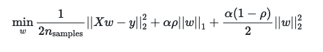
Where alpha and p (or l1\_ratio), need to be predetermined. To estimate these parameters, a 5 fold cross validation was used.
The sklearn implementation [ElasticNetCV](https://scikit-learn.org/stable/modules/generated/sklearn.linear_model.ElasticNetCV.html#sklearn.linear_model.ElasticNetCV) was chosen to model this case.
#### Neural Network Regression
Finally, the last technique used to predict collaboration probability was what is called a “Neural Network Regression”.
Here, the [MLPRegressor](https://scikit-learn.org/stable/modules/generated/sklearn.neural_network.MLPRegressor.html#sklearn.neural_network.MLPRegressor) model from sklearn was used. This methodology applies a neural network that trains a backpropagation algorithm, and uses the squared error as the loss function of the network.
The full mathematical description is considered to be out of scope for this study, however, you can learn more about this methodology in [sklearn’s website](https://scikit-learn.org/stable/modules/neural_networks_supervised.html#regression).
#### Node2Vec
Node2Vec is a technique and framework originally developed by [Stanford University](https://arxiv.org/pdf/1607.00653.pdf) by A.Grover and J.Leskovec in 2016, that learns continuous feature representations from networks. To put it simply, it transforms a weighted network formed of nodes and edges, into a tabular representation of each node as a vector of N dimensions, while preserving a wide set of characteristics.
If you wish to learn more about the technical details of the framework, the reading of the [original paper](https://arxiv.org/pdf/1607.00653.pdf) is highly encouraged.
Stanford also makes an implementation available in the official [SNAP website](https://snap.stanford.edu/node2vec/). For this study, [the python implementation of the algorithm was used](https://github.com/aditya-grover/node2vec).
This implementation allows the creation of such vector representations of nodes (.i.e node embeddings), from a list of nodes and their corresponding weighted edges. It also allows for the determination of the number of dimensions this representation will have in the end.
## Analyses and Results
### Link Prediction
#### Basic Statistics
The variable that was of prediction interest, is the number of co-authored documents between two researchers. In the dataset, this column is defined as “rweight”. Rweight, describes the number of such collaborations between two nodes (p1 and p2).
Let us look at the distribution of this variable in our dataset:

Rweight has a mean of 1.25, a standard deviation of 0.99, but also a 75th percentile of 1.00. This means, as shown in the figure, that the variable is very skewed. In fact, most authors only collaborate one time. However, there are outliers, for example, there is a rweight of 56 in one of the rows, which would mean that these two authors co-authored 56 documents together.
#### Cosine Similarity
One additional metric introduced is the cosine similarity between nodes. Taking the node embeddings described in the second part of the study (LINK), it’s possible to calculate the cosine similarity between them, by applying the [cosine distance function](https://docs.scipy.org/doc/scipy-0.14.0/reference/generated/scipy.spatial.distance.cosine.html) between two vectors.
#### Correlations with author collaboration
Since we are looking to predict the number of collaborations between authors. Let us investigate some of the highest correlations between rweight, and the other attributes in the dataset:
The figure below, is a correlation heatmap that describes our dataset.

Looking closely, the attributes that have a higher correlation with the number of collaborations (rweight) are:
* resourceAllocationscore (0.50 correlation score)
* preferentialAttachmentscore (0.32 correlation score)
* adamicAdarscore with (0.29 correlation score)
These are all metrics derived from the original neo4j network LINK . This leads us to believe that some of the calculated network metrics will be very important in describing the collaboration between two authors.
#### Results
Result Summary
| Model | MAE | MSE | RMSE | R^2 |
| ------------------------- | ---- | ---- | ---- | ---- |
| Linear Regression | 0.40 | 0.55 | 0.74 | 0.42 |
| ElasticNet | 0.41 | 0.58 | 0.76 | 0.34 |
| Neural Network Regression | 0.22 | 0.32 | 0.57 | 0.65 |
| Google AutoML © | 0.20 | - | 0.60 | 0.58 |
### Linear Regression
The first model applied, the Linear regression produced the following results:
| Mean Absolute Error (MAE) | 0.4004 |
| ------------------------------ | ------ |
| Mean Squared Error (MSE) | 0.5462 |
| Root Mean Squared Error (RMSE) | 0.7390 |
| R-squared (R^2) | 0.4171 |
Moreover, when looking at the main features and their coefficients (figure below), we can note that the main features used by the linear regression are:
* Resource Allocation Score
* Cosine similarity
* And Topic similarity

### ElasticNet with Cross Validation
Here are the metrics after fitting and ElasticNet with Cross Validation:
| Mean Absolute Error (MAE) | 0.4100 |
| ------------------------------ | ------ |
| Mean Squared Error (MSE) | 0.5820 |
| Root Mean Squared Error (RMSE) | 0.7629 |
| R-squared (R^2) | 0.3789 |
We can also observe the main coefficients used in this model, by plotting its coefficients:

### Neural Network Regression
By applying the Neural Network Regression, the following results were achieved:
| Mean Absolute Error (MAE) | 0.2218 |
| ------------------------------ | ------ |
| Mean Squared Error (MSE) | 0.3237 |
| Root Mean Squared Error (RMSE) | 0.5690 |
| R-squared (R^2) | 0.6545 |
Moreover, we can also observe the fitting of the model with the test set:

### Google AutoML
In addition to the ML methods previously described we also ran our analyses using [Google AutoML tables](https://cloud.google.com/automl-tables). We decided to do this in order to evaluate Google´s service but also as a way to validate our results against a more "packaged" ML service.
The figure below shows a summary of the results in one of our early tests.

### Node2Vec
Taking the edge list of our network, the node2vec algorithm was successfully run. An important detail is that a weighted edge list was feeded into the algorithm.
`python src/main.py --input corona.edgelist --output corona_128.emd --weighted --dimensions=128`
The output of running this algorithm is a table where every row corresponds to a node, and every column corresponds to an embedding (a float) in each dimension. \
---
# Agent Instructions: Querying This Documentation
If you need additional information that is not directly available in this page, you can query the documentation dynamically by asking a question.
Perform an HTTP GET request on the current page URL with the `ask` query parameter:
```
GET https://dataverz.gitbook.io/coronavirus-r-and-d/matchmaking-experiments/process-details.md?ask=
```
The question should be specific, self-contained, and written in natural language.
The response will contain a direct answer to the question and relevant excerpts and sources from the documentation.
Use this mechanism when the answer is not explicitly present in the current page, you need clarification or additional context, or you want to retrieve related documentation sections.